13 Logistic Regression

13.1 Model form

Logistic regression is a special type of GLM. The name is confusing because the objective is classification and not regression. While most examples focus on binary classification, logistic regression also works for multiclass classification.

The model form is as before

\[g(\mathbf{\hat{y}}) = \mathbf{X} \mathbf{\beta}\]

However, now the target $y_i$ is a category. Our objective is to predict a probability of being in each category. For regression, $\hat{y_i}$ can be any number, but now we need $0 \leq \hat{y_i} \leq 1$.

We can use a special link function, known as the standard logistic function, sigmoid, or logit, to force the output to be in this range of $\{0,1\}$.

\[\mathbf{\hat{y}} = g^{-1}(\mathbf{X} \mathbf{\beta}) = \frac{1}{1 + e^{-\mathbf{X} \mathbf{\beta}}}\]

Figure 13.1: Standard Logistic Function

Other link functions for classification problems are possible as well, although the logistic function is the most common. If a problem asks for an alternative link, such as the probit, fit both models and compare the performance.

13.2 Example

Using the auto_claim data, we predict whether or not a policy has a claim. This is also known as the claim frequency.

auto_claim %>% count(CLM_FLAG)

## # A tibble: 2 x 2
##   CLM_FLAG     n
##   <chr>    <int>
## 1 No        7556
## 2 Yes       2740

About 40% do not have a claim while 60% have at least one claim.

set.seed(42)
index <- createDataPartition(y = auto_claim$CLM_FLAG, 
                             p = 0.8, list = F) %>% as.numeric()
auto_claim <- auto_claim %>% 
  mutate(target = as.factor(ifelse(CLM_FLAG == "Yes", 1,0)))
train <-  auto_claim %>% slice(index)
test <- auto_claim %>% slice(-index)

frequency <- glm(target ~ AGE + GENDER + MARRIED + CAR_USE + 
                   BLUEBOOK + CAR_TYPE + AREA, 
                 data=train, 
                 family = binomial(link="logit"))

All of the variables except for the CAR_TYPE and GENDERM are highly significant. The car types SPORTS CAR and SUV appear to be significant, and so if we wanted to make the model simpler we could create indicator variables for CAR_TYPE == SPORTS CAR and CAR_TYPE == SUV.

frequency %>% summary()

## 
## Call:
## glm(formula = target ~ AGE + GENDER + MARRIED + CAR_USE + BLUEBOOK + 
##     CAR_TYPE + AREA, family = binomial(link = "logit"), data = train)
## 
## Deviance Residuals: 
##     Min       1Q   Median       3Q      Max  
## -1.8431  -0.8077  -0.5331   0.9575   3.0441  
## 
## Coefficients:
##                      Estimate Std. Error z value Pr(>|z|)    
## (Intercept)        -3.523e-01  2.517e-01  -1.400  0.16160    
## AGE                -2.289e-02  3.223e-03  -7.102 1.23e-12 ***
## GENDERM            -1.124e-02  9.304e-02  -0.121  0.90383    
## MARRIEDYes         -6.028e-01  5.445e-02 -11.071  < 2e-16 ***
## CAR_USEPrivate     -1.008e+00  6.569e-02 -15.350  < 2e-16 ***
## BLUEBOOK           -4.025e-05  4.699e-06  -8.564  < 2e-16 ***
## CAR_TYPEPickup     -6.687e-02  1.390e-01  -0.481  0.63048    
## CAR_TYPESedan      -3.689e-01  1.383e-01  -2.667  0.00765 ** 
## CAR_TYPESports Car  6.159e-01  1.891e-01   3.256  0.00113 ** 
## CAR_TYPESUV         2.982e-01  1.772e-01   1.683  0.09240 .  
## CAR_TYPEVan        -8.983e-03  1.319e-01  -0.068  0.94569    
## AREAUrban           2.128e+00  1.064e-01  19.993  < 2e-16 ***
## ---
## Signif. codes:  0 '***' 0.001 '**' 0.01 '*' 0.05 '.' 0.1 ' ' 1
## 
## (Dispersion parameter for binomial family taken to be 1)
## 
##     Null deviance: 9544.3  on 8236  degrees of freedom
## Residual deviance: 8309.6  on 8225  degrees of freedom
## AIC: 8333.6
## 
## Number of Fisher Scoring iterations: 5

The signs of the coefficients tell if the probability of having a claim is either increasing or decreasing by each variable. For example, the likelihood of an accident

Decreases as the age of the car increases
Is lower for men
Is higher for sports cars and SUVs

The p-values tell us if the variable is significant.

Age, MarriedYes, CAR_USEPrivate, BLUEBOOK, and AreaUrban are significant.
Certain values of CAR_TYPE are significant but others are not.

The output is a predicted probability. We can see that this is centered around a probability of about 0.5.

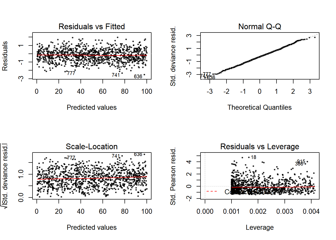
preds <- predict(frequency, newdat=test,type="response")
qplot(preds)

Figure 13.2: Distribution of Predicted Probability

In order to convert these values to predicted 0’s and 1’s, we assign a cutoff value so that if $\hat{y}$ is above this threshold we use a 1 and 0 othersise. The default cutoff is 0.5. We change this to 0.3 and see that there are 763 policies predicted to have claims.

test <- test %>% mutate(pred_zero_one = as.factor(1*(preds>.3)))
summary(test$pred_zero_one)

##    0    1 
## 1296  763

How do we decide on this cutoff value? We need to compare cutoff values based on some evaluation metric. For example, we can use accuracy.

\[\text{Accuracy} = \frac{\text{Correct Guesses}}{\text{Total Guesses}}\]

This results in an accuracy of 70%. But is this good?

test %>% summarise(accuracy = mean(pred_zero_one == target))

## # A tibble: 1 x 1
##   accuracy
##      <dbl>
## 1    0.699

Consider what would happen if we just predicted all 0’s. The accuracy is 74%.

test %>% summarise(accuracy = mean(0 == target))

## # A tibble: 1 x 1
##   accuracy
##      <dbl>
## 1    0.734

For policies which experience claims the accuracy is 63%.

test %>% 
  filter(target == 1) %>% 
  summarise(accuracy = mean(pred_zero_one == target))

## # A tibble: 1 x 1
##   accuracy
##      <dbl>
## 1    0.631

But for policies that don’t actually experience claims this is 72%.

test %>% 
  filter(target == 0) %>% 
  summarise(accuracy = mean(pred_zero_one == target))

## # A tibble: 1 x 1
##   accuracy
##      <dbl>
## 1    0.724

How do we know if this is a good model? We can repeat this process with a different cutoff value and get different accuracy metrics for these groups. Let’s use a cutoff of 0.6.

75%

test <- test %>% mutate(pred_zero_one = as.factor(1*(preds>.6)))
test %>% summarise(accuracy = mean(pred_zero_one == target))

## # A tibble: 1 x 1
##   accuracy
##      <dbl>
## 1    0.752

10% for policies with claims and 98% for policies without claims.

test %>% 
  filter(target == 1) %>% 
  summarise(accuracy = mean(pred_zero_one == target))

## # A tibble: 1 x 1
##   accuracy
##      <dbl>
## 1    0.108

test %>% 
  filter(target == 0) %>% 
  summarise(accuracy = mean(pred_zero_one == target))

## # A tibble: 1 x 1
##   accuracy
##      <dbl>
## 1    0.985

The punchline is that the accuracy depends on the cutoff value, and changing the cutoff value changes whether the model is accuracy for the “true = 1” classes (policies with actual claims) vs. the “false = 0” classes (policies without claims).

13.3 Classification metrics

For regression problems, when the output is a whole number, we can use the sum of squares $\text{RSS}$, the r-squared $R^2$, the mean absolute error $\text{MAE}$, and the likelihood. For classification problems where the output is in $\{0,1\}$, we need to a new set of metrics.

A confusion matrix shows is a table that summarises how the model classifies each group.

No claims and predicted to not have claims - True Negatives (TN) = 1,489
Had claims and predicted to have claims - True Positives (TP) = 59
No claims but predited to have claims - False Positives (FP) = 22
Had claims but predicted not to - False Negatives (FN) = 489

confusionMatrix(test$pred_zero_one,factor(test$target))$table

##           Reference
## Prediction    0    1
##          0 1489  489
##          1   22   59

These definitions allow us to measure performance on the different groups.

Precision answers the question “out of all of the positive predictions, what percentage were correct?”

\[\text{Precision} = \frac{\text{TP}}{\text{TP} + \text{FP}}\]

Recall answers the question “out of all of positive examples in the data set, what percentage were correct?”

\[\text{Recall} = \frac{\text{TP}}{\text{TP} + \text{FN}}\]

The choice of using precision vs. recall depends on the relative cost of making a FP or a FN error. If FP errors are expensive, then use precision; if FN errors are expensive, then use recall.

Example A: the model trying to detect a deadly disease, which only 1 out of every 1000 patient’s survive without early detection. Then the goal should be to optimize recall, because we would want every patient that has the disease to get detected.

Example B: the model is detecting which emails are spam or not. If an important email is flagged as spam incorrectly, the cost is 5 hours of lost productivity. In this case, precision is the main concern.

In some cases we can compare this “cost” in actual values. For example, if a federal court is predicting if a criminal will recommit or not, they can agree that “1 out of every 20 guilty individuals going free” in exchange for “90% of those who are guilty being convicted”. When money is involed, this a dollar amount can be used: flagging non-spam as spam may cost $100 whereas missing a spam email may cost $2. Then the cost-weighted accuracy is

\[\text{Cost} = (100)(\text{FN}) + (2)(\text{FP})\]

Then the cutoff value can be tuned in order to find the minimum cost.

Fortunately, all of this is handled in a single function called confusionMatrix.

confusionMatrix(test$pred_zero_one,factor(test$target))

## Confusion Matrix and Statistics
## 
##           Reference
## Prediction    0    1
##          0 1489  489
##          1   22   59
##                                           
##                Accuracy : 0.7518          
##                  95% CI : (0.7326, 0.7704)
##     No Information Rate : 0.7339          
##     P-Value [Acc > NIR] : 0.03366         
##                                           
##                   Kappa : 0.1278          
##                                           
##  Mcnemar's Test P-Value : < 2e-16         
##                                           
##             Sensitivity : 0.9854          
##             Specificity : 0.1077          
##          Pos Pred Value : 0.7528          
##          Neg Pred Value : 0.7284          
##              Prevalence : 0.7339          
##          Detection Rate : 0.7232          
##    Detection Prevalence : 0.9607          
##       Balanced Accuracy : 0.5466          
##                                           
##        'Positive' Class : 0               
##

13.3.1 Area Under the ROC Curv (AUC)

What if we look at both the true-positive rate (TPR) and false positive rate (FPR) simultaneously? That is, for each value of the cutoff, we can calculate the TPR and TNR.

For example, say that we have 10 cutoff values, $\{k_1, k_2, ..., k_{10}\}$. Then for each value of $k$ we calculate both the true positive rates

\[\text{TPR} = \{\text{TPR}(k_1), \text{TPR}(k_2), .., \text{TPR}(k_{10})\} \]

and the true negative rates

\[\{\text{FNR} = \{\text{FNR}(k_1), \text{FNR}(k_2), .., \text{FNR}(k_{10})\}\]

Then we set x = TPR and y = FNR and graph x against y. The plot below shows the ROC for the auto_claims data. The Area Under the Curv of 0.6795 is what we would get if we integrated under the curve.

library(pROC)
roc(test$target, preds, plot = T)

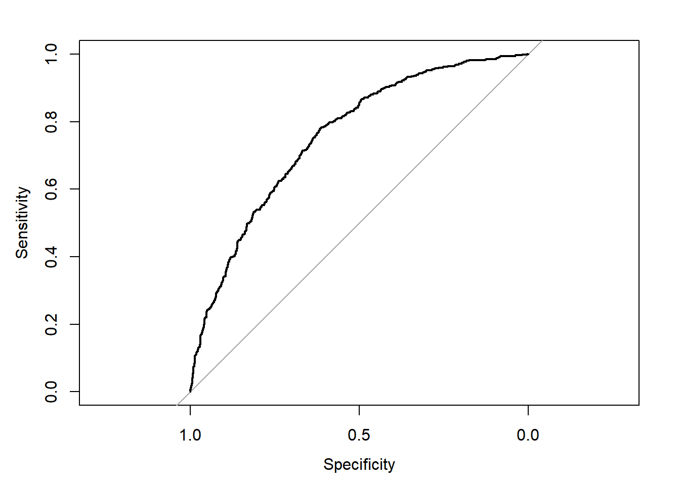
Figure 13.3: AUC for auto_claim

## 
## Call:
## roc.default(response = test$target, predictor = preds, plot = T)
## 
## Data: preds in 1511 controls (test$target 0) < 548 cases (test$target 1).
## Area under the curve: 0.7558

If we just randomly guess, the AUC would be 0.5, which is represented by the 45-degree line. A perfect model would maximize the curve to the upper-left corner.

AUC is preferred over Accuracy when there are a lot more “true” classes than “false” classes, which is known as having **class imbalance*. An example is bank fraud detection: 99.99% of bank transactions are “false” or “0” classes, and so optimizing for accuracy alone will result in a low sensitivity for detecting actual fraud.

13.3.2 Additional reading

Title	Source
An Overview of Classification	ISL 4.1
Understanding AUC - ROC Curv	Sarang Narkhede, Towards Data Science
Precision vs. Recall	Shruti Saxena, Towards Data Science