9 Generalized linear Models (GLMs)
Already enrolled? Watch the full video: Practice Exams + Lessons
GLMs are a broad category of models. Ordinary Least Squares and Logistic Regression are both examples of GLMs.
9.0.1 Assumptions of OLS
We assume that the target is Gaussian with a mean equal to the linear predictor. This can be broken down into two parts:
A random component: The target variable \(Y|X\) is normally distributed with mean \(\mu = \mu(X) = E(Y|X)\)
A link between the target and the covariates (also known as the systemic component) \(\mu(X) = X\beta\)
This says that each observation follows a normal distribution that has a mean that is equal to the linear predictor. Another way of saying this is that “after we adjust for the data, the error is normally distributed and the variance is constant.” If \(I\) is an n-by-in identity matrix, and \(\sigma^2 I\) is the covariance matrix, then
\[ \mathbf{Y|X} \sim N( \mathbf{X \beta}, \mathbf{\sigma^2} I) \]
9.0.2 Assumptions of GLMs
GLMs are more general which eludes that they are more flexible. We relax these two assumptions by saying that the model is defined by
A random component: \(Y|X \sim \text{some exponential family distribution}\)
A link: between the random component and covariates:
\[g(\mu(X)) = X\beta\] where \(g\) is called the link function and \(\mu = E[Y|X]\).
Each observation follows some type of exponential distribution (Gamma, Inverse Gaussian, Poisson, Binomial, etc.), and that distribution has a mean which is related to the linear predictor through the link function. Additionally, there is a dispersion parameter, but that is more info is needed here. For an explanation, see Ch. 2.2 of CAS Monograph 5.
9.1 Advantages and disadvantages
There is usually at least one question on the PA exam which asks you to “list some of the advantages and disadvantages of using this particular model,” and so here is one such list. It is unlikely that the grader will take off points for including too many comments and so a good strategy is to include everything that comes to mind.
GLM Advantages
- Easy to interpret
- Can easily be deployed in spreadsheet format
- Handles different response/target distributions
- Is commonly used in insurance ratemaking
GLM Disadvantages
- Does not select features (without stepwise selection)
- Strict assumptions around distribution shape and randomness of error terms
- Predictor variables need to be uncorrelated
- Unable to detect non-linearity directly (although this can manually be addressed through feature engineering)
- Sensitive to outliers
- Low predictive power
9.2 GLMs for regression
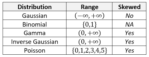
For regression problems, we try to match the actual distribution to the distribution of the model being used in the GLM. These are the most likely distributions.
The choice of target distribution should be similar to the actual distribution of \(Y\). For instance, if \(Y\) is never less than zero, then using the Gaussian distribution is not ideal because this can allow for negative values. If the distribution is right-skewed, then the Gamma or Inverse Gaussian may be appropriate because they are also right-skewed.
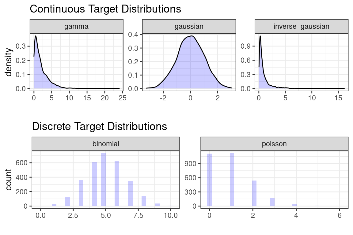
Notice that the top three distributions are continuous but the bottom two are discrete.
There are five link functions for a continuous \(Y\), , although the choice of distribution family will typically rule out several of these immediately. The linear predictor (a.k.a., the systemic component) is \(z\) and the link function is how this connects to the expected value of the response.
\[z = X\beta = g(\mu)\]
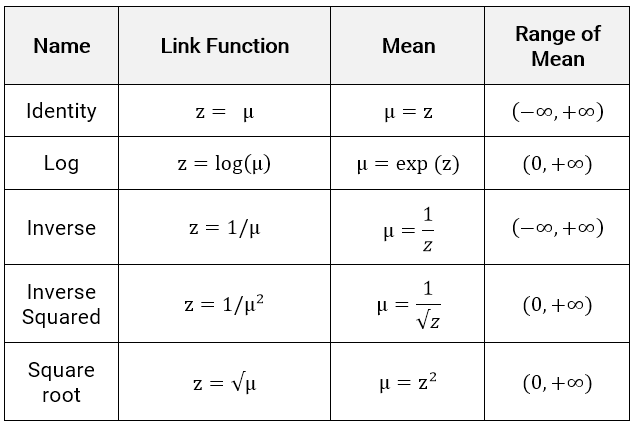
If the target distribution must have a positive mean, such as in the Inverse Gaussian or Gamma, then the Identity or Inverse links are poor choices because they allow for negative values; the mean range is \((-\infty, \infty)\). The other link functions force the mean to be positive.
9.3 Interpretation of coefficients
The GLM’s interpretation depends on the choice of link function.
9.3.1 Identity link
This is the easiest to interpret. For each one-unit increase in \(X_j\), the expected value of the target, \(E[Y]\), increases by \(\beta_j\), assuming that all other variables are held constant.
9.3.2 Log link
This is the most popular choice when the results need to be easy to understand. Simply take the exponent of the coefficients and the model turns into a product of numbers being multiplied together.
\[ log(\hat{Y}) = X\beta \Rightarrow \hat{Y} = e^{X \beta} \]
For a single observation \(Y_i\), this is
\[ \text{exp}(\beta_0 + \beta_1 X_{i1} + \beta_2 X_{i2} + ... + \beta_p X_{ip}) = \\ e^{\beta_0} e^{\beta_1 X_{i1}}e^{\beta_2 X_{i2}} ... e^{\beta_p X_{ip}} = R_{i0} R_{i2} R_{i3} ... R_{ip} \]
\(R_{ik}\) is known as the relativity is known as the relativity of the kth variable. This terminology is from insurance ratemaking, where actuaries need to explain the impact of each variable to insurance regulators.
Another advantage to the log link is that the coefficients can be interpreted as having a percentage change on the target. Here is an example for a GLM with variables \(X_1\) and \(X_2\) and a log link function. This holds any continuous target distribution.
| Variable | \(\beta_j\) | \(e^{\beta_j} - 1\) | Interpretation |
|---|---|---|---|
| (intercept) | 0.100 | 0.105 | |
| \(X_1\) | 0.400 | 0.492 | 49% increase in \(E[Y]\) for each unit increase in \(X_1\)* |
| \(X_2\) | -0.500 | -0.393 | 39% decrease in \(E[Y]\) for each unit increase in \(X_2\)* |
If categorical predictors are used, then the interpretation is very similar. Say that there is one predictor, COLOR, which takes on values of YELLOW (reference level), RED, and BLUE.
| Variable | \(\beta_j\) | \(e^{\beta_j} - 1\) | Interpretation |
|---|---|---|---|
| (intercept) | 0.100 | 0.105 | |
| Color=RED | 0.400 | 0.492 | 49% increase in \(E[Y]\) for RED cars as opposed to YELLOW cars* |
| Color=BLUE | -0.500 | -0.393 | 39% decrease in \(E[Y]\) for BLUE cars rather than YELLOW cars* |
* Assuming all other variables are held constant.
Warning: Never take the log of Y with a GLM! This is a common mistake because we handled skewness for multiple linear regression models, but that was before we had the GLM in our toolbox. Do not move on until you understand the difference between these two models:
glm(y ~ x, family = gaussian(link = “log”), data = data)
glm(log(y) ~ x, family = gaussian(link = “identity”), data = data)
The first says that the target has a Gaussian distribution which has a mean equal to the log of the linear predictor. The second says that the target’s log has a Guassian distribution that is exactly equal to the linear predictor. You will remember from Exam P that when you apply a transform to a random variable, the distribution changes completely. Try running the above examples on real data and see if you can spot the differences in the results.
9.4 Other links
The other link functions are not straightforward to interpret using math. One solution is to use the model-demo-method. See the example at the end of this next chapter.