15 Tree-based models

The models up to this point have been linear. This means that $Y$ changes gradually as $X$ changes.

Tree-based models allow for abrupt changes in $Y$.

Already enrolled? Watch the full video: Practice Exams + Lessons

15.1 Decision Trees

Decision trees can be used for either classification or regression problems. The model structure is a series of yes/no questions. Depending on how each observation answers these questions, a prediction is made.

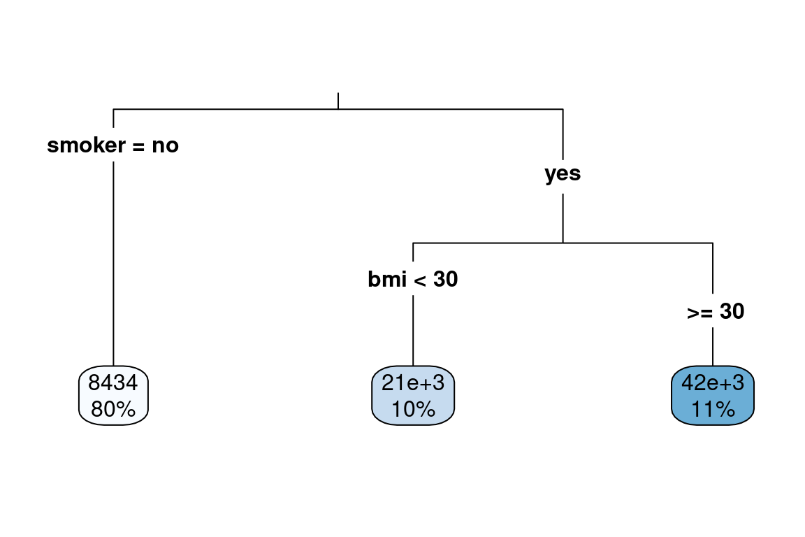
The below example shows how a single tree can predict health claims.

For non-smokers, the predicted annual claims are 8,434. This represents 80% of the observations
For smokers with a bmi of less than 30, the predicted annual claims are 21,000. 10% of patients fall into this bucket.
For smokers with a bmi of more than 30, the prediction is 42,000. This bucket accounts for 11% of patients.

We can cut the data set up into these groups and look at the claim costs. From this grouping, we can see that smoker is the most important variable as the difference in average claims is about 20,000.

smoker	bmi_30	mean_claims	percent
no	bmi < 30	$7,155.75	0.34
no	bmi >= 30	$8,438.77	0.47
yes	bmi < 30	$23,332.61	0.07
yes	bmi >= 30	$42,111.82	0.12

This was a very simple example because there were only two variables. If we have more variables, the tree will get large very quickly. This will result in overfitting; there will be a good performance on the training data but poor performance on the test data.

The step-by-step process of building a tree is

Step 1: Find the best predictor-split-point combination

This variable could be any one of age, children, charges, sex, smoker, age_bucket, bmi, or region.

The split point which best separates observations out based on the value of $y$. A good split is one where the $y$’s are very different. * **

In this case, smoker was chosen. Then it can be only split in one way: smoker = "yes" or smoker = "no". Notice that although this is a categorical variable, the tree does not need to binanize the variables. Instead, like the table above shows, the data gets partitioned by the categories directly.

Then, for each of these groups, smokers and non-smokers find the next variable and split point that best separates the claims. In this case, for no-smokers, age was chosen. To find the best cut point of age, look at all possible age cut points from 18, 19, 20, 21, …, 64 and choose the one which best separates the data.

There are three ways of deciding where to split

Entropy (aka, information gain)
Gini
Classification error

Of these, just the first two are commonly used. The exam is not going to ask you to calculate either of these. It is important to remember that neither method will work better on all data sets, and so the best practice is to test both and compare the performance.

Step 2: Continue doing this until a stopping criterion is reached. For example, the minimum number of observations is 5 or less.

As you can see, this results in a very deep tree.

tree <- rpart(formula = charges ~  ., data = health_insurance,
              control = rpart.control(cp = 0.003))
rpart.plot(tree, type = 3)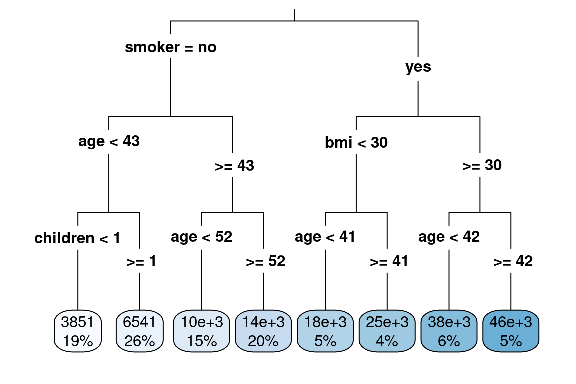

Step 3: Apply cost complexity pruning to simplify the tree

Intuitively, we know that the above model would perform poorly due to overfitting. We want to make it simpler by removing nodes. This is very similar to how linear models reduce complexity by reducing the number of coefficients.

A measure of the depth of the tree is the complexity. A simple way of measuring this from the number of terminal nodes, called $|T|$. In the above example, $|T| = 8$. The amount of penalization is controlled by $\alpha$. This is very similar to $\lambda$ in the Lasso.

Intuitively, only looking at the number of nodes by itself is too simple because not all data sets will have the same characteristics such as $n$, $p$, the number of categorical variables, correlations between variables, and so on. In addition, if we just looked at the error (squared error in this case), we would overfit very easily. To address this issue, we use a cost function that takes into account the error and $|T|$.

To calculate the cost of a tree, number the terminal nodes from $1$ to $|T|$, and let the set of observations that fall into the $mth$ bucket be $R_m$. Then add up the squared error over all terminal nodes to the penalty term.

\[ \text{Cost}_\alpha(T) = \sum_{m=1}^{|T|} \sum_{R_m}(y_i - \hat{y}_{Rm})^2 + \alpha |T| \]

Step 4: Use cross-validation to select the best alpha

The cost is controlled by the CP parameter. In the above example, did you notice the line rpart.control(cp = 0.003)? This is telling rpart to continue growing the tree until the CP reaches 0.003. At each subtree, we can measure the cost CP as well as the cross-validation error xerror.

This is stored in the cptable

tree <- rpart(formula = charges ~  ., data = health_insurance,
              control = rpart.control(cp = 0.0001))
cost <- tree$cptable %>% 
  as_tibble() %>% 
  select(nsplit, CP, xerror) 

cost %>% head()

## # A tibble: 6 × 3
##   nsplit      CP xerror
##    <dbl>   <dbl>  <dbl>
## 1      0 0.620    1.00 
## 2      1 0.144    0.382
## 3      2 0.0637   0.238
## 4      3 0.00967  0.175
## 5      4 0.00784  0.169
## 6      5 0.00712  0.163

As more splits are added, the cost continues to decrease, reaches a minimum, and then begins to increase.

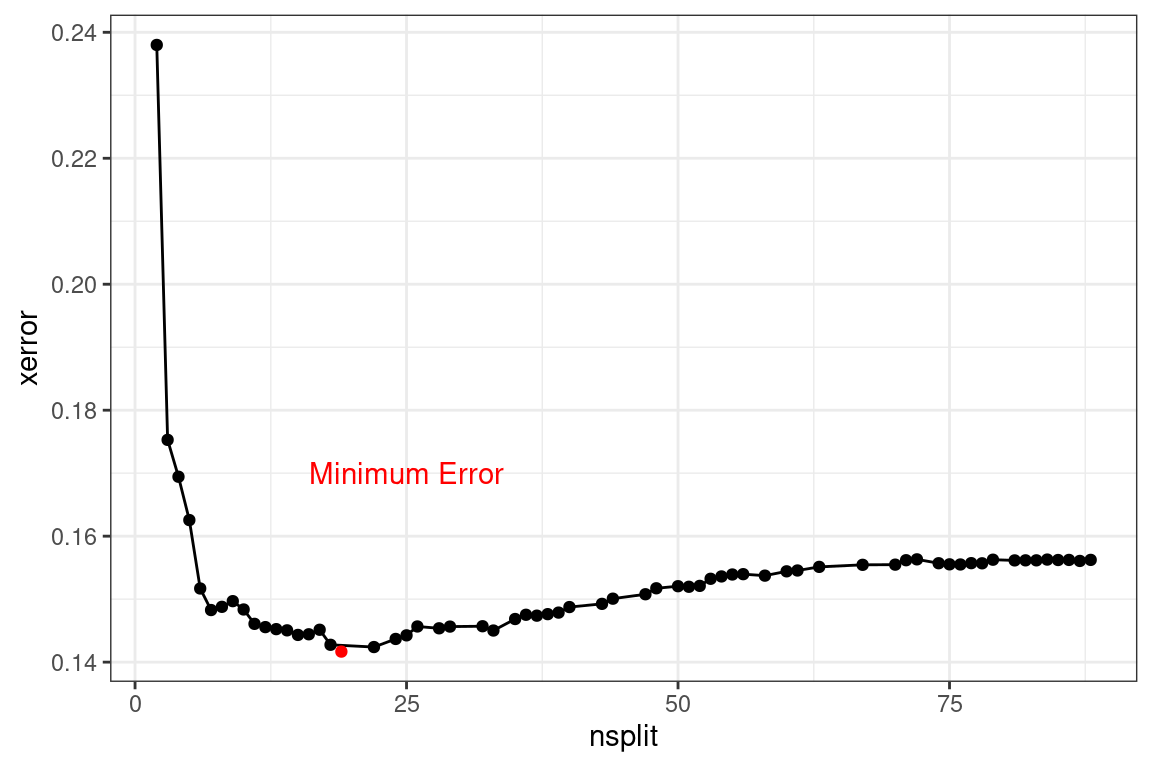
To optimize performance, choose the number of splits that have the lowest error. The goal of using a decision tree is to create a simple model. In this case, we can error the side of a lower nsplit so that the tree is shorter and more interpretable. So far, all of the questions have only used decision trees for interpretability, and a different model method has been used when predictive power is needed.

Once we have selected $\alpha$, the tree is pruned. This table below shows 6 different trees. The xerror column is the missclassification error. The rel error is the relative error, which is the missclassification error divided by its smallest value. This rescales xerror so that the tree with the smallest error is given a rel error of 1.00.

tree$cptable %>% 
  as_tibble() %>% 
  select(nsplit, CP, xerror, `rel error`) %>% 
  head()

## # A tibble: 6 × 4
##   nsplit      CP xerror `rel error`
##    <dbl>   <dbl>  <dbl>       <dbl>
## 1      0 0.620    1.00        1    
## 2      1 0.144    0.382       0.380
## 3      2 0.0637   0.238       0.236
## 4      3 0.00967  0.175       0.173
## 5      4 0.00784  0.169       0.163
## 6      5 0.00712  0.163       0.155

The SOA may give you code to find the lowest CP value, such as below. You could always find this value yourself by inspecting the CP table and choosing the value of CP which has the lowest xerror.

pruned_tree <- prune(tree,
                     cp = tree$cptable[which.min(tree$cptable[, "xerror"]), "CP"])

To make a simple tree, there are a few options

Set the maximum depth of a tree with maxdepth
Manually set cp to be higher
Use fewer input variables and avoid categories with many levels
Force a high number of minimum observations per terminal node with minbucket

For instance, using these suggestions allows for a simpler tree to be fit.

library(caret)
set.seed(42)
index <- createDataPartition(y = health_insurance$charges, 
                             p = 0.8, list = F)
train <- health_insurance %>% slice(index)
test <- health_insurance %>% slice(-index)

simple_tree <- rpart(formula = charges ~  ., 
              data = train,
              control = rpart.control(cp = 0.0001, 
                                      minbucket = 200,
                                      maxdepth = 10))
rpart.plot(simple_tree, type = 3)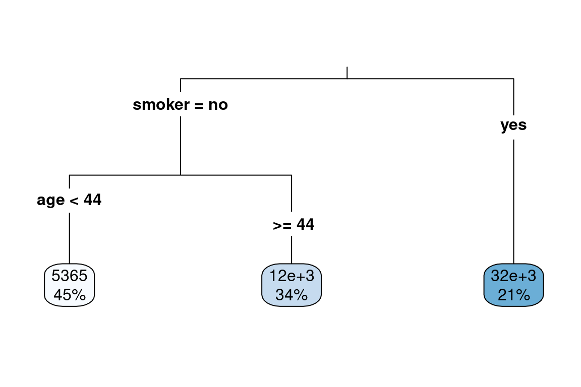

We evaluate the performance on the test set. Because the target variable charges are highly skewed, we use the Root Mean Squared Log Error (RMSLE). We see that the thorny tree has the best (lowest) error and has 8 terminal nodes. The simple tree with only three terminal nodes has a worse (higher) error, but this is still an improvement over the mean prediction.

tree_pred <- predict(tree, test)
simple_tree_pred <- predict(simple_tree, test)

get_rmsle <- function(y, y_hat){
  sqrt(mean((log(y) - log(y_hat))^2))
}

get_rmsle(test$charges, tree_pred)

## [1] 0.3920546

get_rmsle(test$charges, simple_tree_pred)

## [1] 0.5678457

get_rmsle(test$charges, mean(train$charges))

## [1] 0.9996513

15.1.1 Example: SOA PA 6/18/2020, Task 6

Describe what pruning does and why it might be considered for this business problem.

Construct an unpruned regression tree using the code provided.

Review the complexity parameter table and plot for this tree. State the optimal complexity parameter and the number of leaves resulting from the tree pruned using that value.

Prune the tree using a complexity parameter that will result in eight leaves. If eight is not a possible option, select the largest number less than eight that is possible.

Calculate and compare the Pearson goodness-of-fit statistic on the test set for both trees (original and pruned).

Interpret the entire pruned tree (all leaves) in the context of the business problem.

15.1.2 Advantages and disadvantages

Advantages

Easy to interpret
Performs variable selection
Categorical variables do not require binarization in order for each level to be used as a separate predictor
Captures non-linearities
Captures interaction effects
Handles missing values

Disadvantages

Is a “weak learner” because of low predictive power
Does not work on small data sets
Is often a simplification of the underlying process because all observations at terminal nodes have equal predicted values
High variance (which can be alleviated with stricter parameters) leads the “easy to interpret results” to change upon retraining Unable to predict beyond the range of the training data for regression (because each predicted value is an average of training samples)

Readings
ISLR 8.1.1 Basics of Decision Trees
ISLR 8.1.2 Classification Trees
rpart Documentation (Optional)

15.2 Ensemble learning

The “wisdom of crowds” says that often many are smarter than the few. In the context of modeling, the models which we have looked at so far have been single guesses; however, often, the underlying process is more complex than any single model can explain. If we build separate models and then combine them, known as ensembling, performance can be improved. Instead of creating a single perfect model, many simple models, known as weak learners are combined into a meta-model.

The two main ways that models are combined are through bagging and boosting.

15.2.1 Bagging

To start, we create many “copies” of the training data by sampling with replacement. Then we fit a simple model to each data set. Typically is would be a decision tree or linear model because each model is looking at different areas of the data, the predictions are different. The final model is a weighted average of each of the individual models.

15.2.2 Boosting

Boosting always uses the original training data and iteratively fits models to the error of the prior models. These weak learners are ineffective by themselves but powerful when added together. Unlike with bagging, the computer must train these weak learners sequentially instead of in parallel.

15.3 Random Forests

A random forest is the most common example of bagging. As the name implies, a forest is made up of trees. Separate trees are fit to sampled data sets. There is one minor modification for random forests: to make each model even more different; each tree selects a random subset of variables.

If we had to explain why a random forest works in three steps, they would be:

Assume that the underlying process, $Y$, has some signal within the data $\mathbf{X}$.
Introduce randomness (variance) to capture the signal.
Remove the variance by taking an average.

When using only a single tree, there can only be as many predictions as terminal nodes. In a random forest, predictions can be more granular due to the contribution of each of the trees.

The below graph illustrates this. A single tree (left) has stair-like, step-wise predictions, whereas a random forest is free to predict any value. The color represents the predicted value (yellow = highest, black = lowest).

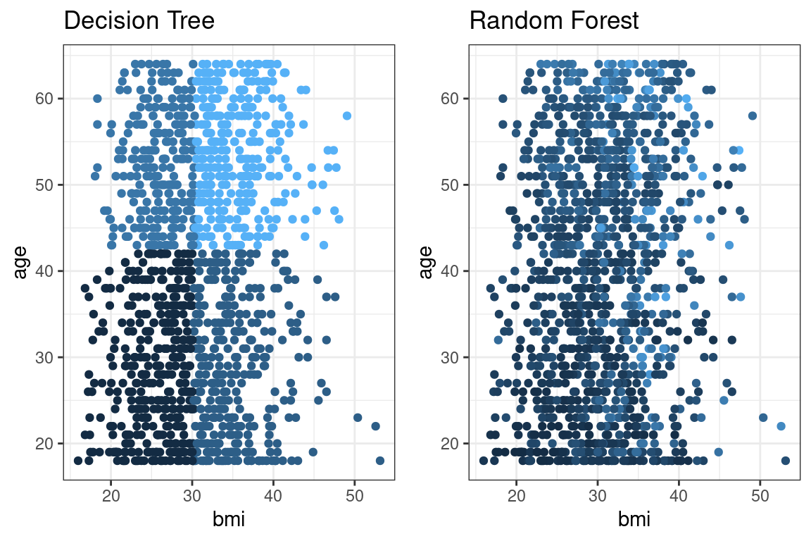
Unlike decision trees, random forest trees do not need to be pruned. Overfitting is less of a problem: if one tree overfits, other trees overfit in other areas to compensate.

In most applications, only the mtry parameter, which controls how many variables to consider at each split, needs to be tuned. Tuning the ntrees parameter is not required; however, the SOA may still ask you to.

15.3.1 Example

Using the basic randomForest package we fit a model with 500 trees.

This expects only numeric values. We create dummy (indicator) columns.

rf_data <- health_insurance %>% 
  sample_frac(0.2) %>% 
  mutate(sex = ifelse(sex == "male", 1, 0),
         smoker = ifelse(smoker == "yes", 1, 0),
         region_ne = ifelse(region == "northeast", 1,0),
         region_nw = ifelse(region == "northwest", 1,0),
         region_se = ifelse(region == "southeast", 1,0),
         region_sw = ifelse(region == "southwest", 1,0)) %>% 
  select(-region)
rf_data %>% glimpse(50)

## Rows: 268
## Columns: 10
## $ age       <dbl> 42, 44, 31, 36, 64, 28, 45, 27…
## $ sex       <dbl> 1, 1, 1, 1, 1, 0, 1, 1, 0, 1, …
## $ bmi       <dbl> 26.125, 39.520, 27.645, 34.430…
## $ children  <dbl> 2, 0, 2, 2, 0, 3, 0, 0, 0, 0, …
## $ smoker    <dbl> 0, 0, 0, 0, 0, 0, 0, 0, 1, 0, …
## $ charges   <dbl> 7729.646, 6948.701, 5031.270, …
## $ region_ne <dbl> 1, 0, 1, 0, 1, 0, 0, 0, 0, 1, …
## $ region_nw <dbl> 0, 1, 0, 0, 0, 1, 1, 0, 1, 0, …
## $ region_se <dbl> 0, 0, 0, 1, 0, 0, 0, 1, 0, 0, …
## $ region_sw <dbl> 0, 0, 0, 0, 0, 0, 0, 0, 0, 0, …

library(caret)
set.seed(42)
index <- createDataPartition(y = rf_data$charges, 
                             p = 0.8, list = F)
train <- rf_data %>% slice(index)
test <- rf_data %>% slice(-index)

rf <- randomForest(charges ~ ., data = train, ntree = 400)
plot(rf)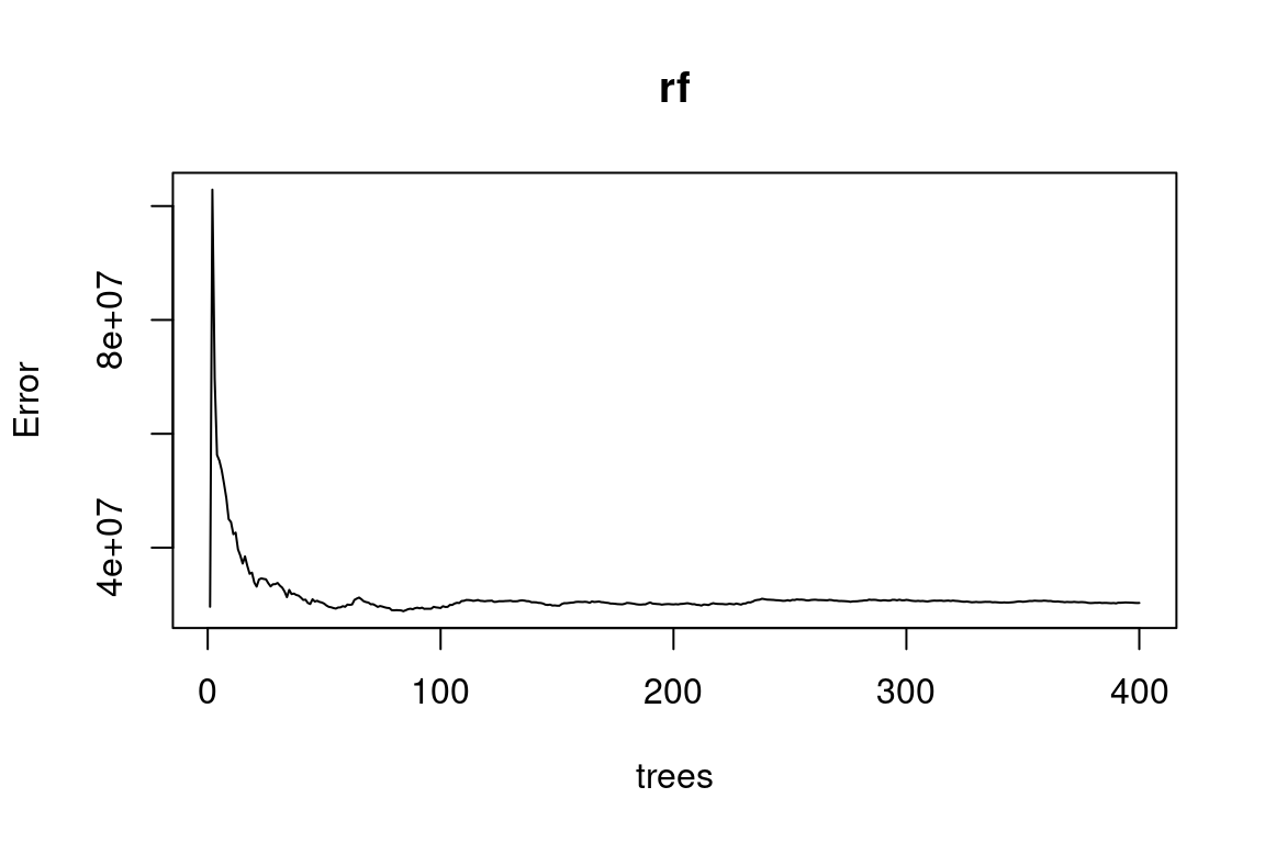

We again use RMSLE. This is lower (better) than a model that uses the average as a baseline.

pred <- predict(rf, test)
get_rmsle <- function(y, y_hat){
  sqrt(mean((log(y) - log(y_hat))^2))
}

get_rmsle(test$charges, pred)

## [1] 0.5252518

get_rmsle(test$charges, mean(train$charges))

## [1] 1.118947

15.3.2 Variable Importance

Variable importance is a way of measuring how each variable contributes to the overall performance of the model. For single decision trees, the variable “higher up” in the tree have greater influence. Statistically, there are two ways of measuring this:

Look at the mean reduction in accuracy when the variable is randomly permuted versus using the actual values from the data. This is done with type = 1 (default).
Use the total decrease in node impurities from splitting on the variable, averaged over all trees. For classification, the node impurity is measured by the Gini index; for regression, it is measured by the residual sum of squares $\text{RSS}$. This is type = 2.

smoker, bmi, and age are the most important predictors of charges. As you can imagine, variable importance is a highly useful tool for building models. We could use this to test out newly engineered features or perform feature selection by taking the top-n features and use them in a different model. Random forests can handle very high dimensional data, which allows for many tests to be run at once.

varImpPlot(x = rf)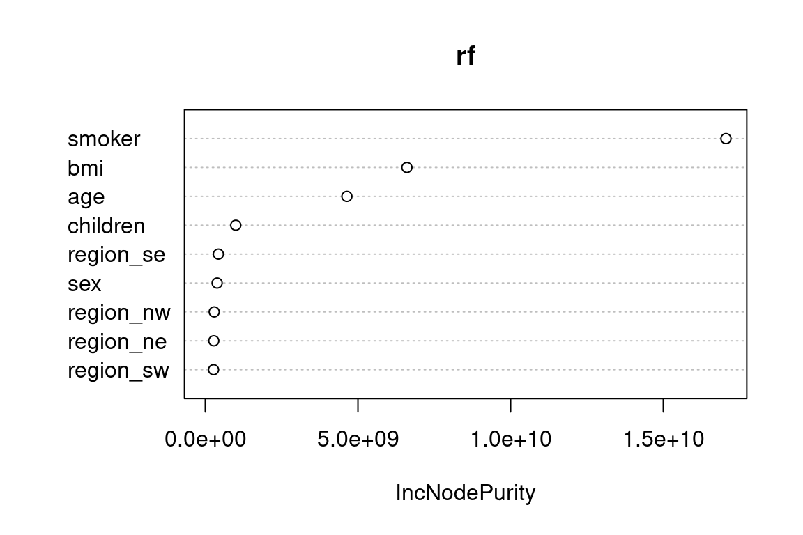

15.3.3 Partial dependence

We know which variables are important, but what about the direction of the change? In a linear model, we would be able to just look at the sign of the coefficient. In tree-based models, we have a tool called partial dependence. This attempts to measure the change in the predicted value by taking the average $\hat{\mathbf{y}}$ after removing the effects of all other predictors.

Although this is commonly used for trees, this approach is model-agnostic in that any model could be used.

Take a model of two predictors, $\hat{\mathbf{y}} = f(\mathbf{X}_1, \mathbf{X_2})$. For simplicity, say that $f(x_1, x_2) = 2x_1 + 3x_2$.

The data looks like this

df <- tibble(x1 = c(1,1,2,2), x2 = c(3,4,5,6)) %>% 
  mutate(f = 2*x1 + 3*x2)
df

## # A tibble: 4 × 3
##      x1    x2     f
##   <dbl> <dbl> <dbl>
## 1     1     3    11
## 2     1     4    14
## 3     2     5    19
## 4     2     6    22

Here is the partial dependence of x1 on to f.

df %>% group_by(x1) %>% summarise(f = mean(f))

## # A tibble: 2 × 2
##      x1     f
##   <dbl> <dbl>
## 1     1  12.5
## 2     2  20.5

This method of using the mean is know as the Monte Carlo method. There are other methods for partial dependence that are not on the syllabus.

For the Random Forest, this is done with pdp::partial().

library(pdp)
bmi <- pdp::partial(rf, pred.var = "bmi", 
                    grid.resolution = 15) %>% 
  autoplot() + theme_bw()
age <- pdp::partial(rf, pred.var = "age", 
                    grid.resolution = 15) %>% 
  autoplot() + theme_bw()

ggarrange(bmi, age)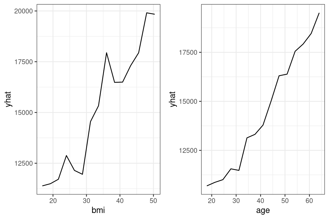

Figure 15.1: Partial Dependence

15.3.4 Advantages and disadvantages

Advantages

Resilient to overfitting due to bagging
• Only one parameter to tune (mtry, the number of features considered at each split)
Very good a multi-class prediction
Nonlinearities
Interaction effects
Handles missing data
Deals with unbalanced after over/undersampling

Disadvantages

Does not work on small data sets
Weaker performance than other methods (GBM, NN)
Unable to predict beyond training data for regression

Readings
ISLR 8.2.1 Bagging
ISLR 8.1.2 Random Forests

15.4 Gradient Boosted Trees

Another ensemble learning method is gradient boosting, also known as the Gradient Boosted Machine (GBM). This is one of the most widely-used and powerful machine learning algorithms that are in use today.

Before diving into gradient boosting, understanding the AdaBoost algorithm is helpful.

15.4.1 Gradient Boosting

15.4.2 Notation

Start with an initial model, which is just a constant prediction of the mean.

\[f = f_0(\mathbf{x_i}) = \frac{1}{n}\sum_{i=1}^ny_i\]

Then we update the target (what the model is predicting) by subtracting off the previously predicted value.

\[ \hat{y_i} \leftarrow y_i - f_0(\mathbf{x_i})\]

This $\hat{y_i}$ is called the residual. In our example, instead of predicting charges, this would be predicting the residual of $\text{charges}_i - \text{Mean}(\text{charges})$. We now use this model for the residuals to update the prediction.

If we updated each prediction with the prior residual directly, the algorithm would be unstable. To make this process more gradual, we use a learning rate parameter.

At step 2, we have

\[f = f_0 + \alpha f_1\]

Then we go back and fit another weak learner to this residual and repeat.

\[f = f_0 + \alpha f_1 + \alpha f_2\]

We then iterate through this process hundreds or thousands of times, slowly improving the prediction.

Because each new tree is fit to residuals instead of the response itself, the process continuously improves the prediction. As the prediction improves, the residuals get smaller and smaller. In random forests or other bagging algorithms, the model performance is more limited by the individual trees because each only contributes to the overall average. The name is gradient boosting because the residuals are an approximation of the gradient, and gradient descent is how the loss functions are optimized.

Similar to how GLMs can be used for classification problems through a logit transform (aka logistic regression), GBMs can also be used for classification.

15.4.3 Parameters

For random forests, the individual tree parameters do not get tuned. For GBMs, however, these parameters can make a significant difference in model performance.

Boosting parameters:

n.trees: Integer specifying the total number of trees to fit. This is equivalent to the number of iterations and the number of basis functions in the additive expansion. Default is 100.
shrinkage: a shrinkage parameter applied to each tree in the expansion. Also known as the learning rate or step-size reduction, 0.001 to 0.1 usually works. A lower learning rate typically requires more trees. Default is 0.1.

Tree parameters:

interaction.depth: Integer specifying the maximum depth of each tree (i.e., the highest level of variable interactions allowed). A value of 1 implies an additive model, a value of 2 implies a model with up to 2-way interactions, etc. Default is 1.
n.minobsinnode: Integer specifying the minimum number of observations in the terminal nodes of the trees. Note that this is the actual number of observations, not the total weight.

GBMs are easy to overfit, and the parameters need to be carefully tuned using cross-validation. In the Examples section, we go through how to do this.

Tip: Whenever fitting a model, use ?model_name to get the documentation. The parameters below are from ?gbm.

15.4.4 Example

We fit a gbm below without tuning the parameters for the sake of example.

library(gbm)
gbm <- gbm(charges ~ ., data = train,
           n.trees = 100,
           interaction.depth = 2,
           n.minobsinnode = 50,
           shrinkage = 0.1)

## Distribution not specified, assuming gaussian ...

pred <- predict(gbm, test, n.trees = 100)

get_rmsle(test$charges, pred)

## [1] 1.052716

get_rmsle(test$charges, mean(train$charges))

## [1] 1.118947

15.4.5 Advantages and disadvantages

This exam covers the basics of GBMs. There are many variations of GBMs not covered in detail, such as xgboost.

Advantages

High prediction accuracy
Shown to work empirically well on many types of problems
Nonlinearities, interaction effects, resilient to outliers, corrects for missing values
Deals with class imbalance directly by weighting observations

Disadvantages

Requires large sample size
Longer training time
Does not detect linear combinations of features. These must be engineered Can overfit if not tuned correctly

Readings
ISLR 8.2.3 Boosting

15.5 Exercises

library(ExamPAData)
library(tidyverse)

Run this code on your computer to answer these exercises.

15.5.1 1. RF tuning with `caret`

The best practice of tuning a model is with cross-validation. This can only be done in the caret library. If the SOA asks you to use caret, they will likely ask you a question related to cross-validation as below.

An actuary has trained a predictive model, chosen the best hyperparameters, cleaned the data, and performed feature engineering. However, they have one problem: the error on the training data is far lower than on new, unseen test data. Read the code below and determine their problem. Find a way to lower the error on the test data without changing the model or the data. Explain the rational behind your method.

set.seed(42)
#Take only 250 records 
#Uncomment this when completing this exercise
data <- health_insurance %>% sample_n(250) 

index <- createDataPartition(
  y = data$charges, p = 0.8, list = F) %>% 
  as.numeric()
train <-  health_insurance %>% slice(index)
test <- health_insurance %>% slice(-index)

control <- trainControl(
  method='boot', 
  number=2, 
  p = 0.2)

tunegrid <- expand.grid(.mtry=c(1,3,5))
rf <- train(charges ~ .,
            data = train,
            method='rf', 
            tuneGrid=tunegrid, 
            trControl=control)

pred_train <- predict(rf, train)
pred_test <- predict(rf, test)

get_rmse <- function(y, y_hat){
  sqrt(mean((y - y_hat)^2))
}

get_rmse(pred_train, train$charges)
get_rmse(pred_test, test$charges)

15.5.2 2. Tuning a GBM with `caret`

If the SOA asks you to tune a GBM, they will need to give you starting hyperparameters that are close to the “best” values due to how slow the Prometric computers are. Another possibility is that they pre-train a GBM model object and ask that you use it.

This example looks at 135 combinations of hyper parameters.

library(caret)
set.seed(42)
index <- createDataPartition(y = health_insurance$charges, 
                             p = 0.8, list = F)
#To make this run faster, only take 50% sample
df <- health_insurance %>% sample_frac(0.50) 
train <- df %>% slice(index) 
test <- df %>% sample_frac(0.05)%>% slice(-index)

tunegrid <- expand.grid(
    interaction.depth = c(1,5, 10),
    n.trees = c(50, 100, 200, 300, 400), 
    shrinkage = c(0.5, 0.1, 0.0001),
    n.minobsinnode = c(5, 30, 100)
    )
nrow(tunegrid)

control <- trainControl(
  method='repeatedcv', 
  number=5, 
  p = 0.8)

gbm <- train(charges ~ .,
            data = train,
            method='gbm', 
            tuneGrid=tunegrid, 
            trControl=control,
            #Show detailed output
            verbose = FALSE
            )

The output shows the RMSE for each of the 135 models tested.

(Part 1 of 3)

Identify the hyperpameter combination that has the lowest training error.

(Part 2 of 3)

2.Suppose that the optimization measure was RMSE. The below table shows the results from three models. Explain why some sets of parameters have better RMSE than the others.

results <- gbm$results %>% arrange(RMSE)
top_result <- results %>% slice(1)%>% mutate(param_rank = 1)
tenth_result <- results %>% slice(10)%>% mutate(param_rank = 10)
twenty_seventh_result <- results %>% slice(135)%>% mutate(param_rank = 135)

rbind(top_result, tenth_result, twenty_seventh_result) %>% 
  select(param_rank, 1:5)

The partial dependence of bmi onto charges makes it appear as if charges increases monotonically as bmi increases.

pdp::partial(gbm, pred.var = "bmi", grid.resolution = 15, plot = T)

However, when we add in the ice curves, we see that there is something else going on. Explain this graph. Why are there two groups of lines?

pdp::partial(gbm, pred.var = "bmi", grid.resolution = 20, plot = T, ice = T, alpha = 0.1, palette = "viridis")

Solutions:

Already enrolled? Watch the full video: Practice Exams | Practice Exams + Lessons

15 Tree-based models

15.1 Decision Trees

15.1.1 Example: SOA PA 6/18/2020, Task 6

15.1.2 Advantages and disadvantages

15.2 Ensemble learning

15.2.1 Bagging

15.2.2 Boosting

15.3 Random Forests

15.3.1 Example

15.3.2 Variable Importance

15.3.3 Partial dependence

15.3.4 Advantages and disadvantages

15.4 Gradient Boosted Trees

15.4.1 Gradient Boosting

15.4.2 Notation

15.4.3 Parameters

15.4.4 Example

15.4.5 Advantages and disadvantages

15.5 Exercises

15.5.1 1. RF tuning with caret

15.5.2 2. Tuning a GBM with caret

15.5.1 1. RF tuning with `caret`

15.5.2 2. Tuning a GBM with `caret`