11 Classification metrics
For regression problems, when the output is a whole number, we can use the sum of squares \(\text{RSS}\), the r-squared \(R^2\), the mean absolute error \(\text{MAE}\), and the likelihood. For classification problems we need to a new set of metrics.
A confusion matrix shows is a table that summarizes how the model classifies each group.
- No claims and predicted to not have claims - True Negatives (TN) = 1,489
- Had claims and predicted to have claims - True Positives (TP) = 59
- No claims but predicted to have claims - False Positives (FP) = 22
- Had claims but predicted not to - False Negatives (FN) = 489
confusionMatrix(test$pred_zero_one,factor(test$target))$table## Reference
## Prediction 0 1
## 0 1489 489
## 1 22 59These definitions allow us to measure performance on the different groups.
Precision answers the question “out of all of the positive predictions, what percentage were correct?”
\[\text{Precision} = \frac{\text{TP}}{\text{TP} + \text{FP}}\]
Recall answers the question “out of all of positive examples in the data set, what percentage were correct?”
\[\text{Recall} = \frac{\text{TP}}{\text{TP} + \text{FN}}\]
The choice of using precision vs. recall depends on the relative cost of making an FP or an FN error. If FP errors are expensive, then use precision; if FN errors are expensive, then use recall.
Example A: the model is trying to detect a deadly disease, which only 1 out of every 1,000 patients survives without early detection. Then the goal should be to optimize recall because we would want every patient that has the disease to get detected.
Example B: the model is detecting which emails are spam or not. If an important email is flagged as spam incorrectly, the cost is 5 hours of lost productivity. In this case, precision is the main concern.
In some cases, we can compare this “cost” in actual values. For example, if a federal court is predicting if a criminal will recommit or not, they can agree that “1 out of every 20 guilty individuals going free” in exchange for “90% of those who are guilty being convicted.”
A dollar amount can be used when money is involved: flagging non-spam as spam may cost $100, whereas missing a spam email may cost $2. Then the cost-weighted accuracy is
\[\text{Cost} = (100)(\text{FN}) + (2)(\text{FP})\]
The cutoff value can be tuned in order to find the minimum cost.
Fortunately, all of this is handled in a single function called confusionMatrix.
confusionMatrix(test$pred_zero_one,factor(test$target))## Confusion Matrix and Statistics
##
##           Reference
## Prediction    0    1
##          0 1489  489
##          1   22   59
##
## Accuracy : 0.7518
## 95% CI : (0.7326, 0.7704)
## No Information Rate : 0.7339
## P-Value [Acc > NIR] : 0.03366
##
## Kappa : 0.1278
##
## Mcnemar's Test P-Value : < 2e-16
##
## Sensitivity : 0.9854
## Specificity : 0.1077
## Pos Pred Value : 0.7528
## Neg Pred Value : 0.7284
## Prevalence : 0.7339
## Detection Rate : 0.7232
## Detection Prevalence : 0.9607
## Balanced Accuracy : 0.5466
##
## 'Positive' Class : 0
## 11.1 Area Under the ROC Curve (AUC)
What if we look at both the true-positive rate (TPR) and false-positive rate (FPR) simultaneously? That is, for each value of the cutoff, we can calculate the TPR and TNR.
For example, say that we have 10 cutoff values, \(\{k_1, k_2, ..., k_{10}\}\). Then for each value of \(k\) we calculate both the true positive rates
\[\text{TPR} = \{\text{TPR}(k_1), \text{TPR}(k_2), .., \text{TPR}(k_{10})\} \]
and the true negative rates
\[\{\text{FNR} = \{\text{FNR}(k_1), \text{FNR}(k_2), .., \text{FNR}(k_{10})\}\]
Then we set x = TPR and y = FNR and graph x against y. The resulting plot is called the Receiver Operator Curve (ROC) and the the Area Under the Curve is called the AUC.
You can also think of AUC as being a probability. Unlike a conventional probability, this ranges between 0.5 and 1 instead of 0 and 1. In the Logit example, we were predicting whether or not an auto policy would file a claim. Then you can interpret the AUC as
The expected proportion of positives ranked before a uniformly drawn random negative
The probability that a model prediction for a policy that filed a claim is greater than the model prediction for a policy that did not file a claim
The expected true positive rate if the ranking is split just before a uniformly drawn random negative.
The expected proportion of negatives ranked after a uniformly drawn random positive.
The expected false positive rate if the ranking is split just after a uniformly drawn random positive.
You can save yourself time by memorizing these three scenarios:
\[ \text{AUC} = 1.0 \]
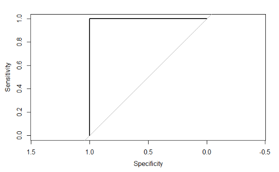
This is a perfect model that predicts the correct class for new data each time. It will have a ROC plot showing the curve approaching the top left corner so that the square area is 1.0.
\[ \text{AUC} = 0.5 \]*
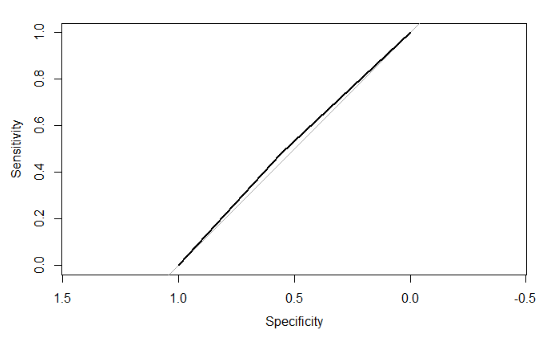
When the ROC curve runs along the diagonal, then the area is 0.5. This performance is no better than randomly selecting the class for new data such that the proportions of each class match that of the data.
\[ \text{AUC} < 0.5 \] Any model having an AUC less than 0.5 means providing predictions that are worse than random selection, with a near 0 AUC indicating that the model makes the wrong classification almost every time. This can occur in two ways
The model is overfitting. For example, the AUC on the train data set may be higher than 0.8 but only 0.2 on the test data set. This indicates that you need to adjust the parameters of your model. See the chapter on the Bias-Variance Tradeoff.
There is an error in the AUC calculation or model prediction.
11.2 Example - Auto Claims
Let’s create an ROC curve and find the AUC for our logit.
library(pROC)
roc(test$target, preds, plot = T)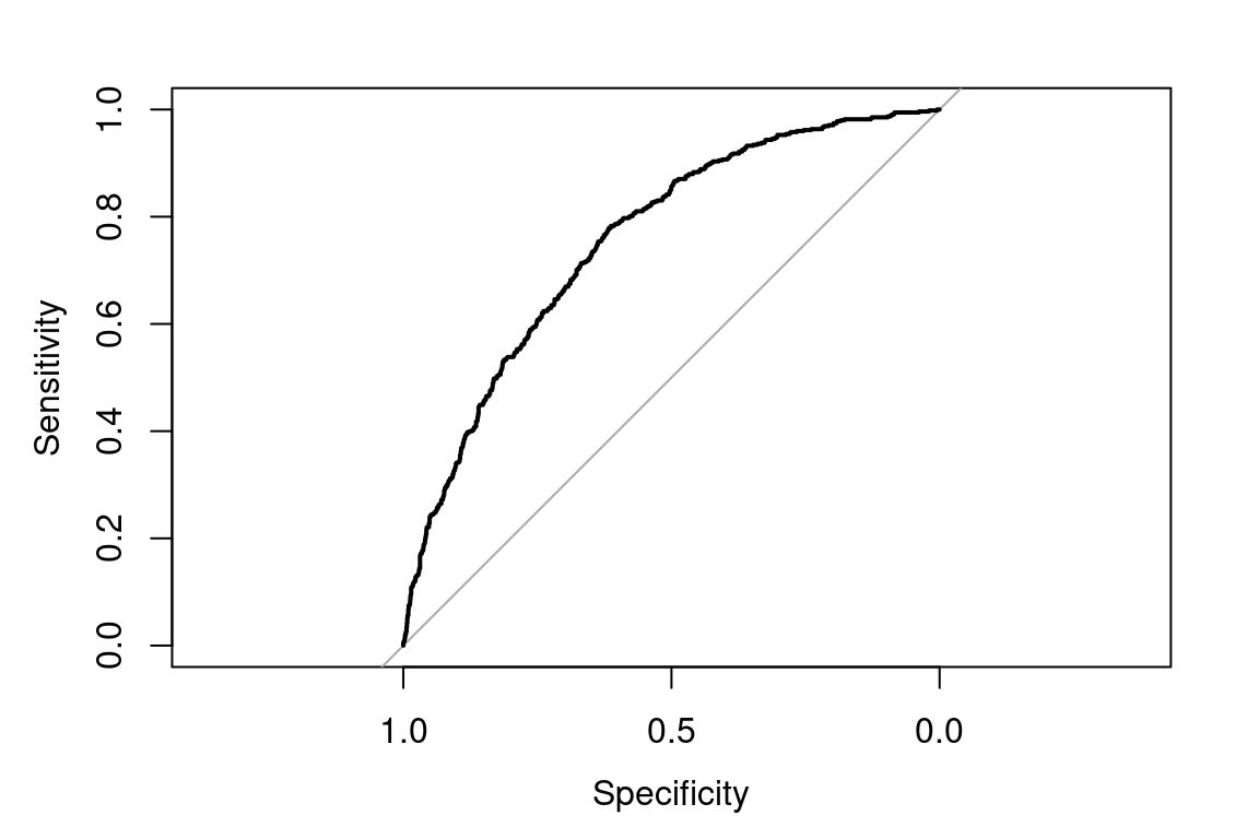
Figure 11.1: AUC for auto_claim
##
## Call:
## roc.default(response = test$target, predictor = preds, plot = T)
##
## Data: preds in 1511 controls (test$target 0) < 548 cases (test$target 1).
## Area under the curve: 0.7558
If we just randomly guess, the AUC would be 0.5, represented by the 45-degree line. A perfect model would maximize the curve to the upper-left corner.
The AUC of 0.76 is decent. If we had multiple models, we could compare them based on the AUC.
In general, AUC is preferred over Accuracy when there are many more “true” classes than “false” classes, which is known as having class imbalance. An example is bank fraud detection: 99.99% of bank transactions are “false” or “0” classes, and so optimizing for accuracy alone will result in a low sensitivity for detecting actual fraud.
11.3 Example: SOA HR, Task 5
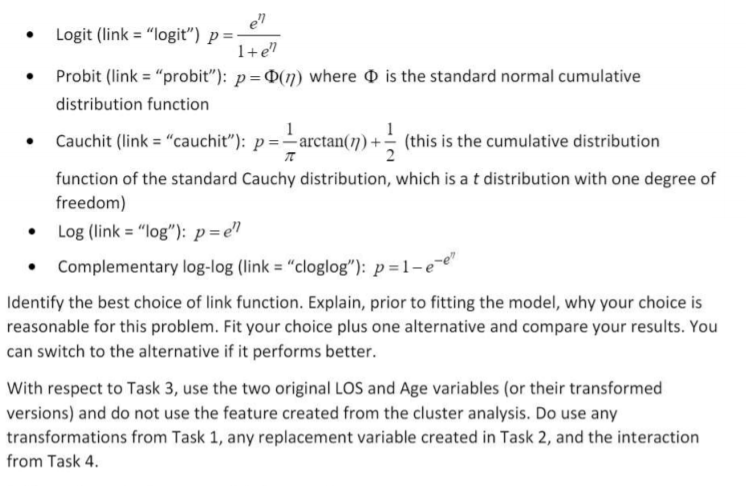
The following question is from the Hospital Readmissions sample project from 2018.
"With the target variable being only 0 or 1, the binomial distribution is the only reasonable choice. Your assistant has done some research and learned that for the glm package in R, five link functions could be used with the binomial distribution. They are shown below (the inverse of the link function is presented here as it represents how the linear predictor is transformed into the actual response), where \(\nu\) is the linear predictor and \(\p\) is the response.
11.4 Example: SOA PA 12/12/19, Task 11
Already enrolled? Watch the full video: Practice Exams | Practice Exams + Lessons
Marketing has asked to demonstrate how your model is to be used with examples of cases that predict high value and cases that predict low value. Your assistant has prepared some sample cases that can be run through your model. You may need to adjust some of them to obtain illustrative examples of interest in marketing.
Write, in language appropriate for marketing, the illustration and demonstration they are looking for. This demonstration should be more detailed than what will go into your executive summary (including an example).
The sample cases are provided here and in your report template if you wish to include them in your report.
probability of each case. You need to create the column Prob of high using your GLM. Then you assign each case as being “High” or “Low” depending on if this value is above the cutoff.
The values that change are in bold.
| age | education num | marital status | occupation | cap_ga in | hours_per week | score | Prob of high | Value |
|---|---|---|---|---|---|---|---|---|
| 39 | 10 | Married-spouse | Group 3 | 0 | 40 | 60 | 0.32 | High |
| 39 | 10 | Never-married | Group 3 | 0 | 40 | 60 | 0.24 | Low |
| 39 | 5 | Married-spouse | Group 3 | 0 | 40 | 60 | 0.39 | High |
| 39 | 10 | Married-spouse | Group 5 | 0 | 40 | 60 | 0.80 | High |
| 39 | 10 | Married-spouse | Group 3 | 0 | 30 | 60 | 0.18 | Low |
You can interpret this as:
- The typical profitable customer is middle aged (39 years old), has 10 years of education, is married, and in group 3
- Having never been married decreases profitability
- Being less educated does not decreases profitability. You can see this because the customer with
education_num = 5has the same characteristics as the first customer - Being in Group 5 increases profitability. You can see this because
Prob of highincreases to 0.8. - Working fewer than 40 hours per week decreases profitability
This was a difficult question. “Do not be afraid to be assertive and think creatively or to change the values that they give you,” the solution of SOA say.
Many candidates struggled with this task. Candidates needed to include sample cases that resulted in low and high-value predictions and clearly describe the analysis for the marketing team.
Candidates were encouraged to modify the supplied cases. Few elected to test changes in both directions from the base case.
11.5 Additional reading
| Title | Source |
|---|---|
| An Overview of Classification | ISL 4.1 |
| Understanding AUC - ROC Curv | Sarang Narkhede, Towards Data Science |
| Precision vs. Recall | Shruti Saxena, Towards Data Science |